Unit 1.3 Water Chemistry, Nutrients And Pollution

Lesson 6/15 | Study Time: 180 Min

Course: Water Science, Management and Governance

Unit 1.3 Water Chemistry, Nutrients And Pollution

Instructor: Mr. Kartik Omanakuttan

In this Unit 1.3, we examine water chemistry as the language of water quality. The unit rewrites and expands the earlier draft of Unit 1.3 so that it follows the instructional rhythm of Units 1.4 to 1.6 while remaining more theoretical and science-led. Governance appears where necessary, but the main emphasis is on chemical processes, nutrient dynamics, pollution pathways, monitoring interpretation, and practical examples.

Water that looks clear may be unsafe. Water that smells unpleasant may or may not be chemically dangerous. A river can carry adequate flow and still fail ecologically because of dissolved oxygen depletion, nutrient enrichment, pathogens, salinity, or toxic contaminants. Chemistry allows us to read what the eye cannot see.

The unit, therefore, asks participants to develop an interpretive skill: to move from a measured value to an explanation of source, pathway, risk, and response. This is the bridge between water science and later units on ecology, groundwater, and irrigation.

1.3.1 Foundations of Water Chemistry and Water Quality

Water chemistry refers to the composition and behaviour of dissolved and suspended substances in water. These include gases such as oxygen and carbon dioxide; major ions such as calcium, magnesium, sodium, chloride, sulfate, and bicarbonate; nutrients such as nitrogen and phosphorus; organic matter; metals; pathogens; synthetic chemicals; microplastics; and emerging contaminants such as pharmaceuticals and endocrine-disrupting compounds. The same water body can be assessed differently depending on use. Drinking water standards focus on human health. Irrigation standards focus on salinity, sodicity, and crop tolerance. Aquatic ecosystem assessment focuses on oxygen, nutrients, temperature, habitat, and toxic stress. Water quality is therefore not a single property but a relationship between chemistry, biology, and purpose.

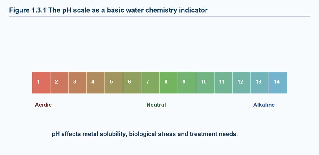
Figure 1.3.1: The pH scale as a basic water chemistry indicator. Source: Kartik Omanakuttan

Several basic parameters appear repeatedly in water science: pH, electrical conductivity, turbidity, temperature, dissolved oxygen, biochemical oxygen demand, nutrients, microbial indicators, and selected toxic chemicals. These parameters are not isolated. Temperature affects oxygen solubility. pH affects metal mobility. Turbidity affects light penetration and treatment. Organic matter affects oxygen demand. Nutrients affect algal growth. Electrical conductivity is a simple but powerful indicator because it reflects the concentration of dissolved ions. High conductivity may indicate natural mineralization, salinity intrusion, irrigation return flows, industrial discharge, or wastewater influence. It does not identify the exact chemical cause, but it warns the investigator that dissolved substances are elevated. pH affects both organisms and chemistry. Many aquatic organisms have limited tolerance ranges. Metals may become more soluble and toxic under some pH conditions. Treatment processes also depend on pH. Therefore, pH is not merely a number on a scale; it influences chemical behaviour and biological risk. Dissolved oxygen is a direct bridge between chemistry and ecology. Fish, invertebrates, and aerobic microbes require oxygen. Oxygen concentration is affected by temperature, turbulence, photosynthesis, respiration, and decomposition of organic matter. A river can look full and still be ecologically stressed if oxygen is depleted.

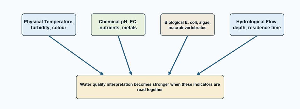
Figure 1.3.2: Indicator groups used in water quality assessment. Source: Kartik Omanakuttan

Read the Bare Fact

Water quality is not a laboratory appendix to water management. It is often the decisive condition. A polluted river is not available in any meaningful sense until it can support the use or ecosystem for which it is needed.

Task and Instructions for Participants

All participants are advised to review the following open-access materials before continuing. As you read, focus on how water quality is defined differently for drinking water, ecosystems, and pollution control.

Essential Watch

Focus on how nitrogen and phosphorus shift from necessary nutrients to pollutants when present in excess.

Additional Watch

Focus on pathogen pollution, organic pollution, salinity and eutrophication.

Narration - The Chemistry of Water as Practical Evidence

The water molecule is simple, but natural water is never only H2O. Rainwater dissolves gases from the atmosphere. Soil water dissolves minerals and organic compounds. Groundwater reflects the chemistry of aquifer materials and residence time. Rivers integrate inputs from soils, vegetation, settlements, farms, drains, and industries. By the time water reaches a monitoring station, its chemistry is a record of the landscape it has travelled through. This is why water chemistry is diagnostic. Elevated nitrate in a shallow well may suggest fertilizer leaching, septic contamination, or manure management problems. High conductivity may indicate salinity, industrial discharge, or return flows from irrigation. High BOD indicates organic pollution that can consume oxygen. Low dissolved oxygen signals stress for fish and other aquatic organisms. High turbidity may indicate erosion, storm runoff, or disturbance of sediments.

1.3.2 Nutrients, Organic Matter and Oxygen Dynamics

Nitrogen and phosphorus are essential nutrients. Without them, aquatic plants and algae cannot grow. The problem begins when nutrient concentrations exceed the capacity of an ecosystem to assimilate them. EPA describes nutrient pollution as too much nitrogen and phosphorus entering air and water, usually from a wide range of human activities; excess nutrients cause algae and algae-like bacteria to grow faster than ecosystems can handle (EPA, 2026).

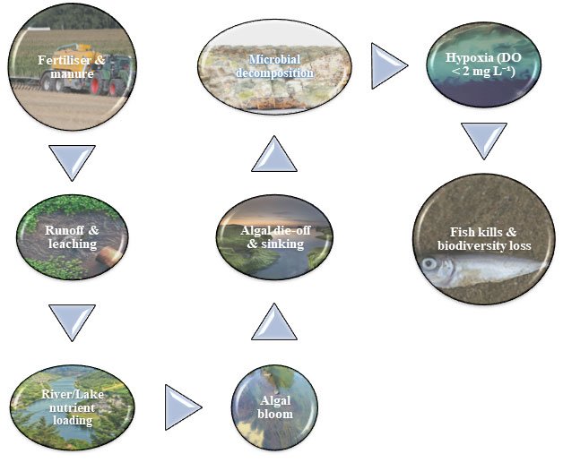
Figure 1.3.3: Nutrient transfer from land to eutrophication. Source: based on EPA (2025) nutrient pollution explanations.

Eutrophication is the enrichment of water with nutrients, leading to increased primary production. The visible symptom may be algal growth. The deeper problem often appears later, when algal biomass dies and decomposes. Microbial decomposition consumes dissolved oxygen, creating hypoxia or even anoxia. Fish and invertebrates may then experience stress, migration, reproductive failure, or mortality.

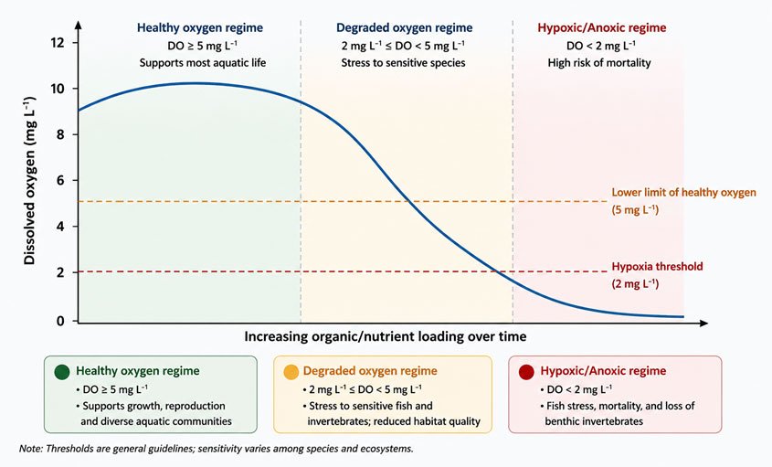
Figure 1.3.4: Nutrient and organic loading can depress dissolved oxygen. Source: Kartik Omanakuttan

Organic pollution follows a related pathway. Sewage, food-processing waste, animal waste and other biodegradable materials increase biochemical oxygen demand. BOD is not itself a pollutant but a measure of the oxygen required by microorganisms to decompose organic matter. High BOD means that oxygen may be depleted, particularly in slow-moving or warm water. Temperature changes the oxygen story. Warm water holds less oxygen than cold water. Therefore, a river receiving the same organic load may experience more severe oxygen stress during hot periods. This is one reason climate change can amplify water quality problems even when pollutant loads remain unchanged. Nutrient limitation is also important. In some freshwater systems, phosphorus is the limiting nutrient; in some coastal systems, nitrogen is more important; in many systems, both matter. A management response that reduces one nutrient but ignores the other may produce incomplete recovery. This is why nutrient control must be based on local monitoring and ecosystem understanding.

Nutrients can also interact with drinking-water treatment. Cyanobacterial blooms may produce toxins such as microcystins. Even when treatment plants are designed for ordinary turbidity and microbial risk, algal toxins can require additional monitoring and treatment processes. Thus, a nutrient problem in a catchment can become a drinking-water problem in a city.

1.3.3 Pollution Pathways and Contaminant Groups

Pollution reaches water through multiple pathways. Point sources discharge through identifiable outlets, such as pipes from sewage treatment plants or industrial facilities. Non-point sources are diffuse, such as fertiliser runoff from farms, sediment from eroding catchments, pesticides from fields, and pollutants washed from urban surfaces during storms. Groundwater contamination may occur through leaching, seepage from waste sites, septic systems, salinisation, or geogenic contaminants such as arsenic and fluoride.

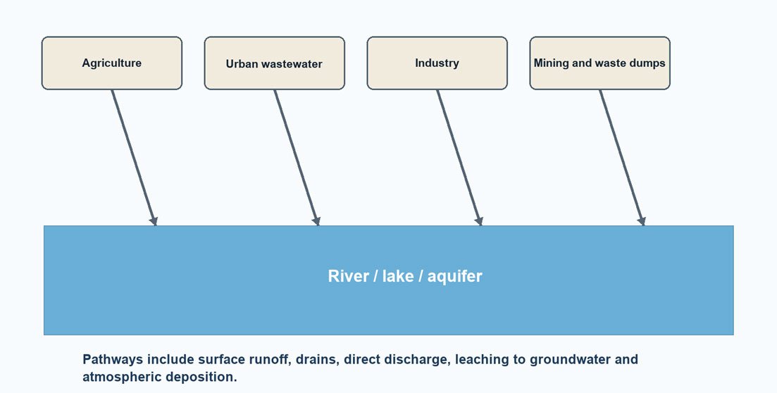
Figure 1.3.5: Common pathways by which pollutants reach water bodies. Source: Kartik Omanakuttan

Major contaminant groups include pathogens, nutrients, organic matter, suspended sediment, salts, metals, pesticides, industrial chemicals, hydrocarbons, pharmaceuticals, and microplastics. UNEP's global water quality assessment highlights pathogen pollution, organic pollution, salinity, and eutrophication as major surface-water concerns in Asia, Africa, and Latin America. Drinking-water risks may be acute or chronic (UNEP, 2016). Pathogens can cause immediate disease outbreaks. Chemical contaminants often produce chronic risks through long-term exposure. WHO (2023) notes that drinking-water safety requires managing risks from catchment to consumer through health-based targets, water safety plans, and surveillance. Some pollutants are conservative, meaning they do not readily degrade or transform under ordinary environmental conditions. Salts and some metals can persist and accumulate. Others are reactive, transforming through biological or chemical processes. Organic matter decomposes. Nitrogen changes form through nitrification and denitrification. Pesticides may degrade into metabolites that have their own risks.

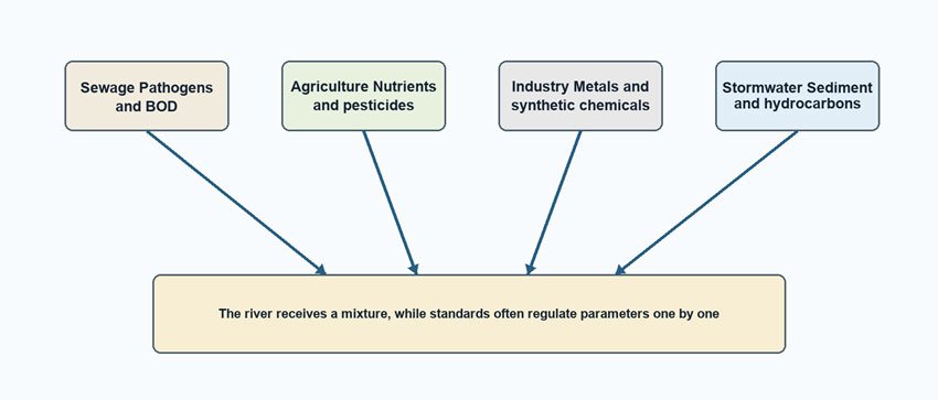
Figure 1.3.6: Mixture risk in a multi-use river. Source: Kartik Omanakuttan

Nitrate in Groundwater

Nitrate is a common groundwater contaminant in agricultural and peri-urban landscapes. It is highly soluble and can move through soil into shallow aquifers. Infants are particularly vulnerable to nitrate in drinking water, and the WHO (2022a) maintains chemical fact sheets and guideline values for nitrate and nitrite in drinking water quality guidance. The practical lesson is that a borewell in a farming region should not be assumed safe merely because the groundwater looks clear. The pathway matters. Nitrate from fertiliser does not always reach groundwater immediately. It may be taken up by crops, retained temporarily in soil, denitrified under suitable conditions, or leached downward during rainfall and irrigation. Monitoring must therefore consider season, crop cycle, soil type, and well depth. Not all contamination comes directly from industrial discharge. Arsenic in groundwater is often geogenic, meaning it is released from natural sediments under particular geochemical conditions. WHO estimates that about 140 million people in at least 70 countries have been drinking water containing arsenic above the provisional guideline value of 10 micrograms per litre. This example shows why water quality assessment must include both human pollution and natural geochemistry. Arsenic also illustrates the danger of assuming that groundwater is naturally safe (WHO, 2022b). In many regions, groundwater was promoted because it was microbiologically safer than surface water. That was often true for diarrhoeal disease, but it did not guarantee chemical safety. A water source can reduce one risk while creating another.

1.3.4 Water Quality Monitoring, Indicators, and Interpretation

Monitoring is the bridge between water chemistry and practical judgement. A water quality number is useful only if we know how the sample was collected, where it was collected, when it was collected, what method was used, and what threshold it is being compared against.

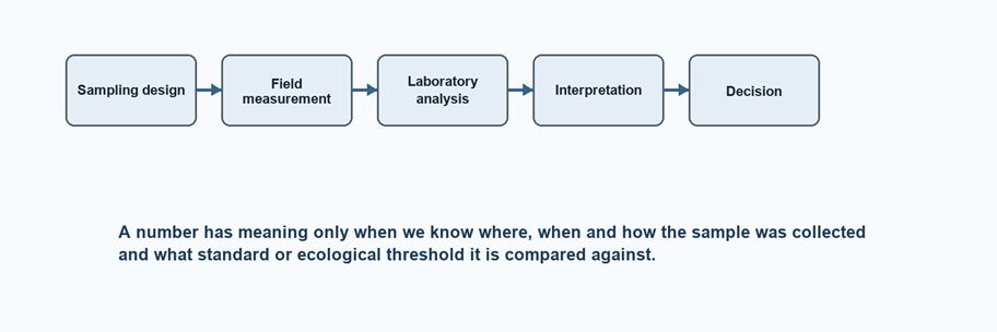
Figure 1.3.7: From water sample to interpretation. Source: Kartik Omanakuttan

Sampling design matters. A sample taken during dry-season baseflow may tell a different story from a sample taken during the first storm after fertiliser application. A sample at the riverbank may differ from a mid-channel sample. A surface sample in a lake may differ from deep water. For groundwater, depth, well construction, pumping duration, and aquifer type all matter. Common field parameters include temperature, pH, electrical conductivity, dissolved oxygen, and turbidity. Laboratory parameters include nutrients, BOD, chemical oxygen demand, metals, pesticides, and microbial indicators. Remote sensing can support assessment of turbidity, chlorophyll-a and surface algal blooms, but it does not replace field and laboratory monitoring. A critical skill is interpretation. High nitrate may signal agricultural leaching, but local septic systems can also contribute. High conductivity may reflect natural geology, irrigation return flows, road salts, or industrial discharge. Low dissolved oxygen may indicate organic loading, thermal pollution, or slow water circulation. Good interpretation, therefore, requires chemistry, hydrology, and local knowledge together. Quality assurance and quality control are not bureaucratic details. Field meters must be calibrated. Samples must be preserved correctly. Holding times must be respected. Chain-of-custody procedures may be necessary for legal or enforcement cases. Duplicate samples and blanks help identify contamination or measurement error. Without QA/QC, monitoring results may create false confidence.

1.3.5 Implications for Human Health and Ecosystems

Chemically and biologically degraded water affects human health, ecosystems, and livelihoods. Pathogen pollution can cause diarrhoeal disease, cholera, typhoid, and other infections. Chemical pollutants can produce chronic health risks. Nutrient pollution can generate harmful algal blooms, some of which produce toxins. Salinity can reduce drinking-water acceptability and damage crops. Heavy metals and persistent organic pollutants can accumulate in organisms and food webs. Ecosystem impacts are equally serious. Low dissolved oxygen reduces habitat quality. High turbidity reduces light penetration and affects aquatic plants. Toxic contaminants can impair reproduction and survival. Nutrient enrichment can shift aquatic communities toward algal dominance. Salinity changes can exclude freshwater species. The important theoretical point is that water quality is cumulative. A river receiving treated wastewater, agricultural runoff, stormwater, sediment, and industrial discharge may not be defined by one pollutant alone. Organisms and people experience mixtures. This complicates monitoring because legal standards may address parameters one by one while ecological stress emerges from combined pressures. Human health risk also depends on exposure. A contaminant in a river may matter differently depending on whether the river is used for drinking, bathing, fishing, irrigation, livestock watering, or cultural practices. Risk assessment, therefore, connects concentration with pathway and population. This is why a technically modest concentration can still matter if exposure is frequent or if the exposed population is vulnerable.

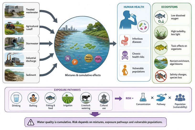
Figure 1.3.8: Impacts of water quality on human health and the ecosystem. Source: Kartik Omanakuttan

Case Study 1.3-A - Lake Winnipeg and Watershed-Scale Nutrient Loading

Lake Winnipeg is one of the world's largest freshwater lakes and has experienced serious eutrophication concerns linked to phosphorus and nitrogen inputs from its extensive watershed. Environment and Climate Change Canada (2024) tracks nutrient levels in Lake Winnipeg and its major tributaries, including the Red, Winnipeg, and Saskatchewan rivers, and links monitoring to phosphorus reduction efforts.

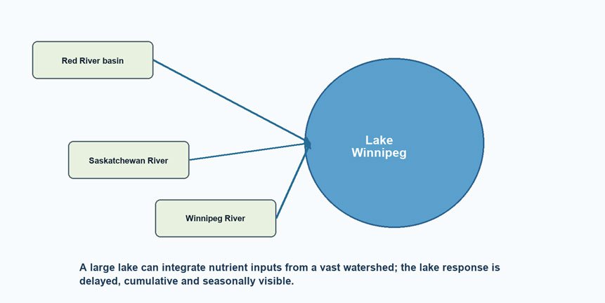
Figure 1.3.9: Lake Winnipeg as a watershed-scale nutrient pollution example. Source: based on Environment and Climate Change Canada (2024)

The scientific lesson from Lake Winnipeg is that lake water quality cannot be understood only at the lake shore. Nutrients arrive through tributaries, land-use practices, urban wastewater, agricultural runoff, and climatic variability. A lake integrates catchment behaviour over time. Large lakes often respond slowly to nutrient reductions because internal loading from sediments may continue and because hydrological residence time is long. This creates a frustrating lag between intervention and visible recovery. Participants should recognise that delayed recovery does not necessarily mean intervention has failed; it may mean that the system has memory. The case also shows why monitoring tributaries matters. If only the lake is monitored, managers see symptoms. If tributaries and land-use changes are monitored, managers begin to see pathways. Good water chemistry is therefore spatially organised: it follows the movement of water and pollutants through the watershed.

Task for Students: Analytical questions from the case study

Participants should answer the following questions in Forum W-001 under the tag "Case Study 1.3".

Why are large lakes especially vulnerable to cumulative nutrient loading?
Which monitoring indicators would you prioritise for diagnosing eutrophication in a lake system?
How can upstream land-use data improve the interpretation of lake water chemistry?

Figure 1.3.10: A man in a polluted river in India. Source: Pexels

Case Study 1.3-B - Polluted River Stretches in India and the Use of BOD as an Indicator

Case Study 1.3-B: Polluted River Stretches in India and the Use of BOD as an Indicator

India's river pollution monitoring system provides an important example of how water quality science is translated into environmental governance. Since 2009, the Central Pollution Control Board (CPCB), in collaboration with State Pollution Control Boards, has periodically assessed river water quality across the country under the National Water Quality Monitoring Programme. One of the principal indicators used to identify polluted river stretches is Biochemical Oxygen Demand (BOD), a measure of the amount of dissolved oxygen required by microorganisms to decompose organic matter in water. High BOD values generally indicate elevated organic pollution from untreated sewage, industrial effluents, agricultural wastes, and other oxygen-consuming substances.

The scale of monitoring is substantial. According to CPCB assessments based on water quality data collected across hundreds of rivers and thousands of monitoring locations, 311 polluted river stretches were identified on 279 rivers in 30 States and Union Territories in the 2022 assessment, compared with 351 polluted stretches identified in 2018. This reduction suggests measurable improvements in some locations and reflects investments in sewage treatment infrastructure, pollution control measures, and river restoration programmes. Nevertheless, the persistence of more than three hundred polluted stretches demonstrates that river pollution remains a major environmental challenge across India.

The scientific importance of BOD lies in its ability to reveal the consequences of organic pollution on aquatic ecosystems. When untreated sewage enters a river, microorganisms begin decomposing the organic material. This decomposition process consumes dissolved oxygen. If oxygen consumption exceeds replenishment from atmospheric exchange and photosynthesis, dissolved oxygen concentrations decline, placing stress on fish, aquatic invertebrates, and other organisms. At sufficiently high BOD levels, rivers can become biologically degraded, supporting only pollution-tolerant species.

The Yamuna River in Delhi provides one of the most widely cited examples. Although the Yamuna contributes only a small proportion of the river's total length within the National Capital Region, this stretch receives a large share of untreated and partially treated wastewater from urban drains. Consequently, BOD concentrations frequently exceed recommended standards, indicating severe organic loading. Similar concerns have been reported in stretches of the Sabarmati, Mithi, Musi, and Satluj rivers, where untreated sewage, industrial discharges, and urban runoff contribute to persistent water-quality deterioration. Recent CPCB assessments continue to identify several stretches where BOD levels remain far above desirable thresholds.

Yet the Indian experience also illustrates the limitations of relying too heavily on a single indicator. BOD was originally developed to assess oxygen-demanding organic pollution, particularly from sewage. It is highly effective for that purpose. However, rivers are increasingly exposed to contaminants that may not substantially influence BOD measurements. Heavy metals from industrial activities, pesticide residues from agriculture, pharmaceutical compounds, microplastics, endocrine-disrupting chemicals, and emerging contaminants can all pose serious ecological and public health risks while producing relatively modest changes in BOD values.

This creates a critical governance challenge. A river stretch may show improvement in BOD and therefore appear to be recovering, while still experiencing contamination from pollutants that are not captured by routine monitoring. For example, a river receiving pesticide runoff may meet BOD targets but still present risks to aquatic biodiversity and drinking-water supplies. Similarly, toxic industrial contaminants can affect ecosystems even when oxygen conditions appear acceptable. In such situations, improvement in one indicator can create a misleading perception of overall improvement.

The issue is not that BOD is scientifically flawed. Rather, it reflects the broader principle that environmental indicators simplify reality. Policymakers require indicators because complex ecosystems cannot be governed using thousands of variables simultaneously. The challenge lies in recognizing what an indicator reveals and what it obscures. BOD reveals organic pollution exceptionally well. It reveals much less about toxicity, nutrient enrichment, pathogen risks, or chemical contamination.

The CPCB itself increasingly employs broader monitoring frameworks incorporating dissolved oxygen, faecal coliforms, pH, conductivity, nutrients, and other parameters. Nevertheless, BOD remains central because untreated sewage continues to be one of the dominant sources of river pollution across much of India. Government assessments note that municipal wastewater remains a major contributor to river degradation, especially in rapidly urbanizing regions where sewage treatment capacity has not kept pace with population growth.

The broader lesson for water science, management, and governance is therefore not simply how to measure pollution, but how to interpret indicators responsibly. River health cannot be reduced to a single number. A scientifically robust monitoring system uses BOD as an entry point rather than a final answer. Initial identification of polluted stretches can be based on BOD, but diagnosis and management require additional parameters selected according to local pollution sources, ecological conditions, and water-use objectives.

Ultimately, the CPCB river monitoring programme demonstrates both the power and limitations of environmental indicators. Indicators make large-scale governance possible. Without them, national assessments of river health would be impractical. However, indicators also shape what governments see, what they prioritise, and what they overlook. Effective water governance, therefore, depends not only on collecting data but on continuously questioning whether the indicators being used are sufficient to capture the changing realities of river pollution.

India's Central Pollution Control Board identifies polluted river stretches using water quality monitoring data, with biochemical oxygen demand as a key indicator of organic pollution. A 2025 Government of India release reports that the CPCB identified 311 polluted river stretches on 279 rivers in 30 States and Union Territories in the 2022 report, down from 351 in 2018.

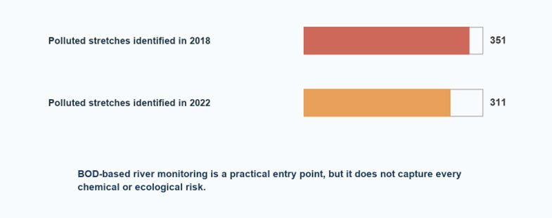
Figure 1.3.11: Polluted river stretches in India identified by CPCB. Source: Based on Press Information Bureau (2025), CPCB reporting.

The scientific lesson is twofold. First, BOD is a practical and useful indicator of organic pollution. Second, it is incomplete. A river stretch may improve in BOD while still facing risks from nutrients, pathogens, metals, pesticides, emerging contaminants, or altered flow. Monitoring programmes must therefore balance simple indicators with broader diagnostic capacity.

BOD-based monitoring is useful because organic pollution remains a major pressure on many rivers. However, if a river is affected by industrial chemicals or agricultural pesticides, BOD alone may understate risk. A scientifically stronger monitoring system uses BOD as one entry point, then adds parameters based on likely sources and uses.

Case Study 1.3-C - Clear Groundwater and Invisible Chemical Risk

In many rural regions, groundwater is trusted because it is visually clear and protected from direct surface contamination. This trust is understandable but incomplete. Groundwater can contain nitrate, fluoride, arsenic, salinity, pesticides, or industrial solvents without obvious taste, colour or smell. A household may therefore prefer groundwater for good reasons and still face chemical risk. The case is not meant to discourage groundwater use. It is meant to discipline interpretation. A safe-looking source must be tested against relevant risks. The relevant risk depends on geology, land use, well depth, sanitation, agriculture, industry, and coastal conditions. A universal testing package may be too expensive, but a risk-based testing package is essential. For understanding this case study, the strongest example is arsenic-contaminated groundwater in Bangladesh and the Bengal Basin, because it perfectly illustrates the central lesson of the section: water can appear clean, safe, and desirable while posing a severe chemical risk that is invisible without testing.

Figure 1.3.12: A tubewell in the middle of a polluted water body. Source: Pexels

Case Study 1.3-C: Clear Groundwater and Invisible Chemical Risk — Arsenic in Bangladesh's Tube Wells

One of the most important lessons in water chemistry and pollution is that water quality cannot be judged by appearance alone. Few examples demonstrate this more clearly than the groundwater arsenic crisis of Bangladesh, widely regarded as one of the largest environmental public health emergencies associated with drinking water in modern history.

Beginning in the 1970s and 1980s, millions of shallow tube wells were installed across rural Bangladesh to provide communities with access to groundwater. At the time, the programme was considered a major public health success. Surface water sources such as ponds, rivers, and canals were frequently contaminated with pathogens responsible for diarrhoeal disease, cholera, and other waterborne illnesses. Groundwater offered an attractive alternative. It was clear, odourless, protected from direct surface contamination, and available close to households. The wells significantly reduced exposure to microbial pathogens and contributed to major improvements in public health.

However, the apparent success concealed a chemical risk that remained largely invisible for years. During the 1990s, scientists discovered that many groundwater sources in the Bengal Basin contained naturally occurring arsenic at concentrations far above recommended drinking-water standards. The contamination was not caused by industrial pollution or poor sanitation. Rather, it originated from geological sediments deposited by the Ganges, Brahmaputra, and Meghna river systems over thousands of years. Under specific geochemical conditions, arsenic was released from these sediments into groundwater and accumulated in shallow aquifers.

The scale of exposure was unprecedented. The World Health Organization described the crisis as "the largest mass poisoning of a population in history." Estimates suggest that between 35 and 77 million people in Bangladesh have been exposed to arsenic-contaminated groundwater, while WHO (2022b) assessments indicate that at least 140 million people globally are exposed to arsenic-contaminated groundwater above recommended limits. Bangladesh and neighbouring regions of India remain among the most severely affected areas.

What made the problem particularly difficult to detect was that arsenic-contaminated groundwater typically appeared entirely normal. The water was colourless, odourless, and often tasted no different from uncontaminated water. Households therefore had little reason to suspect that their preferred source of drinking water posed a hazard. Unlike microbial contamination, which may produce acute illness within days, arsenic exposure is chronic and cumulative. Health effects often emerge only after years or decades of consumption. Long-term exposure has been associated with skin lesions, cancers of the skin, bladder and lungs, cardiovascular disease, neurological disorders, adverse pregnancy outcomes, and reduced cognitive development in children.

The crisis revealed another important scientific insight: contamination is often highly heterogeneous. Wells located only a few metres apart may contain dramatically different arsenic concentrations because groundwater chemistry varies according to local geology, sediment composition, aquifer depth, and groundwater flow paths. In many villages, one well may be safe while a neighbouring well exceeds drinking-water guidelines several times over. This spatial variability means that blanket assumptions about groundwater safety are unreliable and that testing must occur at the scale of individual wells.

The governance implications are equally significant. When arsenic contamination was discovered, responses initially focused on testing wells and marking them with colour codes to distinguish safer sources from contaminated ones. Over time, a wider range of mitigation measures emerged, including deeper wells, piped water systems, community treatment facilities, rainwater harvesting, and groundwater monitoring programmes. Yet implementation proved challenging because technical solutions alone could not overcome issues of affordability, maintenance, institutional capacity, and unequal access. More than two decades after the problem was identified, millions of people continue to rely on contaminated sources because safe alternatives are unavailable, inaccessible, or poorly maintained.

The Bangladesh experience fundamentally changed global thinking about groundwater quality. For decades, groundwater was widely regarded as inherently safer than surface water because it was protected from direct contamination. The arsenic crisis demonstrated that groundwater quality depends not only on sanitation and pollution control but also on geology, hydrogeochemistry, aquifer conditions, and long-term monitoring. Water that appears clean may still contain contaminants capable of causing serious disease.

The broader lesson for water science, management, and governance is therefore not to distrust groundwater, but to interpret it scientifically. Safe-looking water is not necessarily safe water. The relevant risks depend on local geology, land use, agricultural practices, sanitation systems, industrial activities, and coastal processes. Universal testing for every contaminant may be impractical and prohibitively expensive. However, risk-based testing strategies that target contaminants likely to occur in specific settings are essential. Groundwater management must therefore combine hydrogeological understanding, chemical monitoring, public health surveillance, and community engagement if invisible risks are to be identified before they become visible human tragedies.

Task for Students: Discussion Questions

All participants should answer the following quiz questions in Forum W-001. Answer in brief.

Why did communities trust groundwater sources even when arsenic contamination was present?
What makes chemical contamination more difficult to detect than microbial contamination?
Why can neighbouring wells have very different arsenic concentrations?

1.3.7 From Monitoring to Action

Monitoring is only useful if it leads to interpretation and response. A high nitrate value should lead to questions about fertilizer timing, crop uptake, septic systems, manure handling, well depth, and recharge pathways. A low dissolved oxygen value should lead to questions about organic loading, temperature, flow velocity, algal cycles, and wastewater inputs. A high conductivity value should lead to questions about salinity sources, irrigation return flows, and geology.

The response must match the diagnosis. If the source is sewage, treatment and sanitation matter. If the pathway is storm runoff, drainage, and land management matter. If the pollutant is geogenic arsenic, source substitution, treatment, and well testing matter. If the problem is nutrient loading, both wastewater and agricultural land use may need attention.

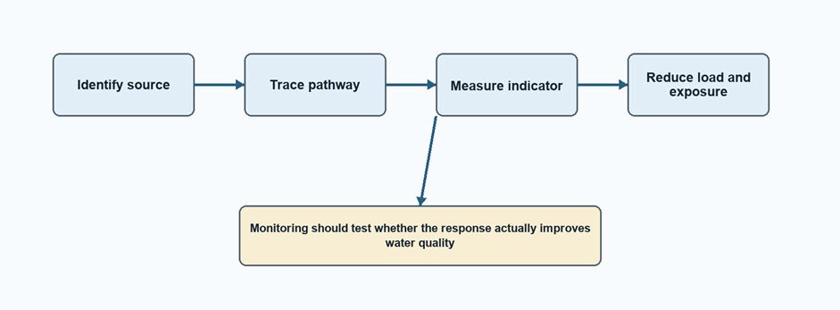
Figure 1.3.13: From pollution diagnosis to practical response. Source: Kartik Omanakuttan

Designing a Practical Monitoring Plan

A practical monitoring plan begins with the question, not the laboratory list. If the question is whether sewage is affecting a river, then BOD, dissolved oxygen, ammoniacal nitrogen, faecal indicator bacteria, and flow conditions may be central. If the question is whether agricultural runoff is affecting a reservoir, then nutrients, turbidity, chlorophyll-a, pesticides, and storm-event sampling may be more relevant. The plan should specify sampling locations. Upstream reference sites help distinguish background conditions from local pollution. Downstream sites show cumulative impact. Tributary sites identify pathways. Drinking-water intake sites connect environmental quality to public health risk. Groundwater sites should be selected by aquifer, depth, and likely contaminant pathway rather than convenience alone. The plan should also specify the sampling frequency. Monthly sampling may miss short pollution pulses. First-flush storm samples may be essential in urban and agricultural catchments. Dry-season samples may reveal concentration under low dilution. Continuous sensors may be needed where dissolved oxygen, temperature, or conductivity changes rapidly. Finally, the plan should state how results will be used. Monitoring that produces reports but no response becomes a ritual. Monitoring should trigger interpretation, communication, enforcement where appropriate, treatment improvements, land-management changes, or further investigation.

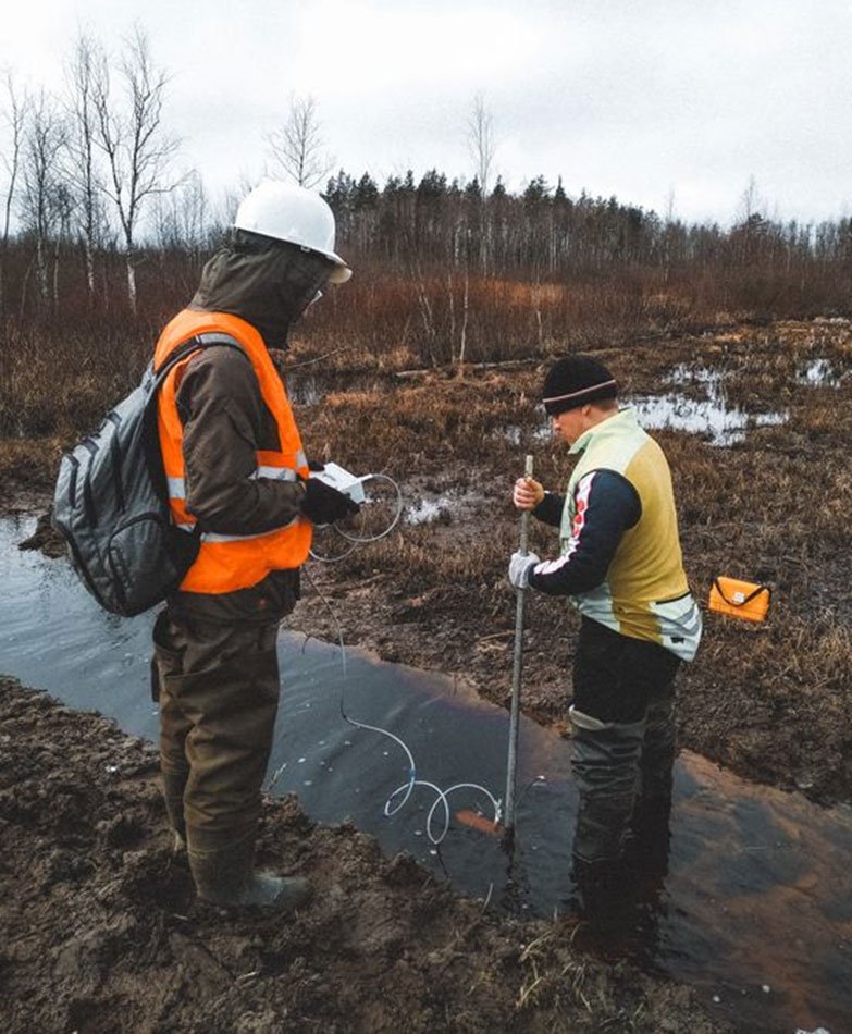
Figure 1.3.14: Researchers performing water monitoring tests. Source: Pexels

Communicating Water Quality to Non-Specialists

Water quality communication is a scientific responsibility. A monitoring agency may understand nitrate, BOD, dissolved oxygen, and faecal coliforms, but the public usually experiences water through colour, smell, taste, illness, fish deaths, crop effects, or official warnings. The task is to translate without oversimplifying. Good communication avoids two extremes. It does not create unnecessary panic when a parameter exceeds an ecological guideline but does not threaten drinking-water safety. It also does not reassure people falsely when clear water contains invisible chemical or microbial risk. The message must specify the use: safe for bathing, unsafe for drinking, suitable for irrigation, harmful for fish, or requiring treatment. Uncertainty should be communicated plainly. If a sample shows high contamination, people should know whether it is a one-time result, a seasonal pattern, a storm-related pulse, or a long-term trend. If further testing is needed, that should be stated directly. Trust is built when scientific limits are made visible.

For course participants, this matters because water quality is often where science meets public anxiety. A good practitioner can read laboratory data, but an excellent practitioner can explain what the data mean for households, farmers, fishers, local governments, and ecosystems.

Case Study 1.3-D: First Flush Pollution and Stormwater Runoff — Combined Sewer Overflows in the River Thames

The River Thames in the United Kingdom provides a useful example of why water quality cannot be understood through routine sampling alone. Over many years, environmental agencies observed that water quality measurements collected during ordinary flow conditions often suggested gradual improvement in river health. However, intense rainfall events revealed a different reality. Much of London's older drainage infrastructure was built as a combined sewer system, where stormwater and wastewater are conveyed through the same network of pipes. During dry weather, wastewater is transported to treatment facilities. During heavy rainfall, however, the volume of incoming water can exceed system capacity. To prevent sewage backing up into streets and homes, excess water is discharged directly into rivers through Combined Sewer Overflows (CSOs).

The first stages of a storm event are particularly important. After a prolonged dry period, pollutants accumulate on roads, rooftops, pavements, and within drainage networks. These include hydrocarbons from vehicles, nutrients, sediments, litter, animal waste, metals, and untreated sewage residues. When rainfall begins, this accumulated material is rapidly washed into receiving waters. The resulting first flush can produce short-lived but intense spikes in contamination that are far greater than concentrations observed during normal conditions. Monitoring of the Thames has shown that storm events can trigger sudden declines in dissolved oxygen and substantial increases in bacterial contamination, creating risks for aquatic organisms and recreational users. In some years, storm overflows have discharged millions of cubic metres of untreated wastewater into the river system. Environmental groups and regulators have increasingly emphasized that assessments based solely on routine dry-weather monitoring underestimate the true pollution burden experienced by rivers.

The Thames case demonstrates a fundamental lesson for water science and management. Water quality depends not only on what is measured but also on when it is measured. A river that appears relatively healthy during baseflow conditions may experience severe pollution during storm events. Event-based monitoring is therefore essential for understanding non-point source pollution, urban runoff, and the environmental impacts of extreme rainfall. The case also illustrates an important connection between hydrology and water chemistry. Pollutant concentrations are often controlled by the timing and magnitude of runoff. Understanding water quality, therefore, requires understanding how water moves through a catchment, particularly during periods of rapid hydrological change.

The first flush is the initial runoff from a rainfall event that washes accumulated pollutants from roads, roofs, drains, fields, and open surfaces into receiving waters. It can contain sediment, hydrocarbons, nutrients, animal waste, litter, metals, and microbial contamination. If monitoring is done only during ordinary dry-weather flow, this pollution pulse may be missed. First-flush pollution is particularly important in cities and peri-urban agricultural areas. A stream may appear relatively clean during baseflow but experience acute contamination during the first major rainfall after a dry period. Aquatic organisms and downstream users experience the pulse even if the monitoring programme does not. The lesson is methodological. Water quality is not only about which parameters are measured; it is also about when they are measured. Event-based sampling is often necessary to understand non-point pollution. This connects Unit 1.3 back to Unit 1.1: hydrological timing controls chemical evidence.

Mandatory Quiz: [Click Here]

1.3.8 Wrap Up Unit 1.3

Please post a short synthesis in Forum W-001 under the tag "Unit 1.3 Reflection". Your response should identify one water quality problem in your region and describe: the likely pollutant, the pathway into water, the monitoring parameter needed, and the potential human or ecological consequence.

Closing Note

Water chemistry teaches humility. A transparent glass can contain nitrate, arsenic, pathogens, or pesticide residues. A green lake can be telling the story of fields far upstream. A low oxygen reading can reveal the invisible work of microbes decomposing yesterday's waste. To read water well, we must learn to read both the molecule and the landscape.

References

Environment and Climate Change Canada (2024). Nutrients in Lake Winnipeg.
EPA (2026). Nutrient pollution overview.
https://www.epa.gov/nutrientpollution/basic-information-nutrient-pollution
EPA (2025). U.S. Environmental Protection Agency—Basic Information on Nutrient Pollution.
NASA Science (n.d.). The Water Cycle.
https://science.nasa.gov/earth/earth-observatory/the-water-cycle
Press Information Bureau, Government of India. (2025). Polluted River Stretches Identified by
CPCB. https://www.pib.gov.in/PressReleseDetailm.aspx?PRID=2155023
UNEP (2016). Hundreds of Millions Face Health Risk as Water Pollution Rises Across Three
USGS Water Science School (2022). Water Cycle Diagrams.
https://www.usgs.gov/special-topics/water-science-school/science/water-cycle-diagrams
WHO (2022a). Chemical fact sheets, nitrate/nitrite.
https://www.who.int/publications/m/item/chemical-fact-sheets--nitrate-nitrite
WHO (2022b). Arsenic fact sheet.
https://www.who.int/news-room/fact-sheets/detail/arsenic
WHO (2023). Drinking-water fact sheet.
https://www.who.int/news-room/fact-sheets/detail/drinking-water